3D Representation 2025.09.03 (Updated: 2025.09.04) computer vision，3D Vision

Comparison between 2D-land and 3D-land

Working with images in 2D feels almost effortless. No matter whether a picture comes from your phone, a DSLR, or an old camera, it always ends up as the same thing: a grid of pixels. This simple, unified representation makes it easy to move images across tools—Photoshop, PyTorch, TensorFlow, you name it. Everything speaks the same language.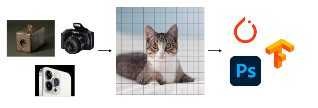

But in 3D, things get messy. There isn’t just one way to represent the world. Instead, we have meshes, point clouds, voxels, implicit surfaces, CAD models, and more. Each has its strengths, but they don’t play well together. A file from one tool often won’t work in another without painful conversions.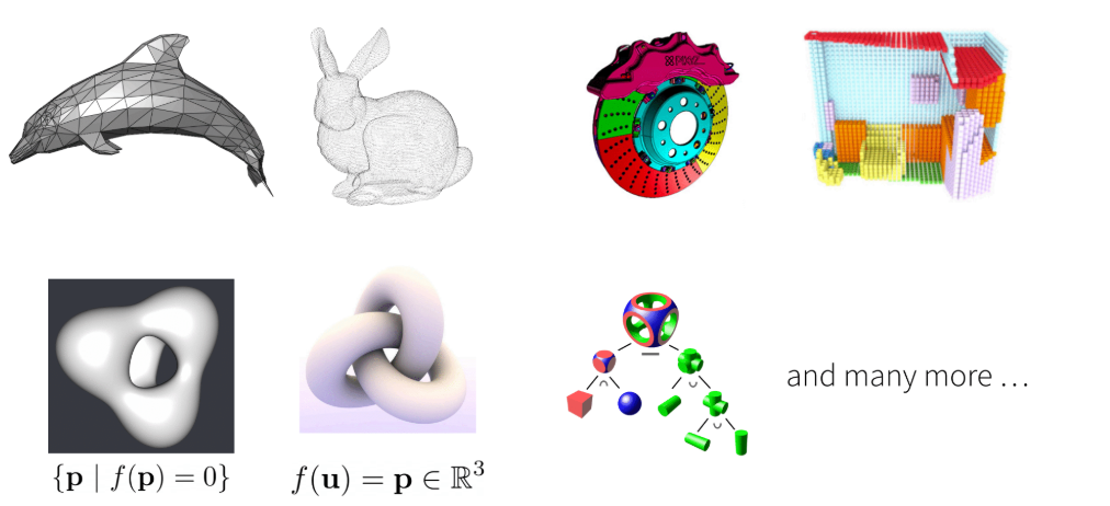

That’s the big difference: 2D has pixels, 3D doesn’t. And until 3D finds its “pixel grid,” working in 3D-land will always feel more fragmented.

So What's the best 3D representation? The answer is that it depends. Acquisition,editing,animation,prediction,optimization will have different prefered representations. In this blog, I will give you a overview of several 3D representations, expressions in code, limitations, benefits and conversions across representations.

Depth Maps

It's an image that represents how far each pixel $\textbf{p}$ is: $D[\textbf{p}]\in \mathbb{R}^+$. It's also expressed in pixel-grid like 2D image where the RGB value in each pixel is replaced with corresponding depth.

We can also extend this representaion to capture other surface properties e.g. surface normals ($N[\textbf{p}]\in \mathbb{S}^2$ where $\mathbb{S}^2 $ is the unit squre.). We can use RGB values to express each surface point's normal vector $(x,y,z)$.

However, the depth map representation is actually 2.5D representation instead of a 3D model. Instead of capturing complete three-dimensional structure, depth maps work by associating depth properties (distance values) to individual image pixels. The representation is fundamentally tied to a particular viewpoint or image perspective. Thus we call it "image-dependent"

Point Clouds

This representation is acquired in an image-like manner from sensors (from mulitple views), but it's not image-dependent. The full 3D structure of the scene can be captured by point clouds. It can also unify approaches independent of sensing modality (i.e. whether the 3D data was captured from LiDAR sensors, stereo cameras... it can be converted into the same point cloud format).

Data structure to store point clouds: they are represented as a $N \times 3$ array where ordering does not matter (i.e. unordered set, unlike images). Each item of the array is a $(x,y,z)$ coordinate of some point. Like the figure shows: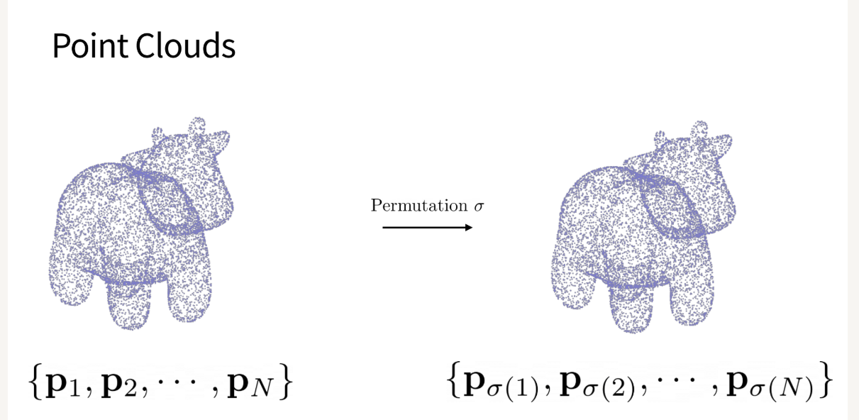

Important features: Since the Permutation Invariance of the point clouds, some processing/generation methods don't work, e.g. CNN and fully connected layer, since they are permutation sensitive. So we need some processing/generation methods that are permutation invariant, e.g. Point Net which will be covered in future notes.

Extensions: Like the extensive version of depth maps can store surface normals, point clouds can also store each point's normal vector if we treat each point as small flat disks instead of tiny spheres. This the unordered set becomes: $\{(\textbf{p}_1,\textbf{n}_1),\dots, (\textbf{p}_N,\textbf{n}_N)\}\in \mathbb{R}^{N\times 6}$. Since we treat points as small flat disks, each disk has one well-defined surface normal. So simple, efficient lighting calculations can be derived using standard dot product operations, thus benefits rendering process.

Limitations: It can be easily observed that it can not explicitly capture connectivity information. So to mostly capture the connectivity information using point clouds representaion, we need to sample more points - but it's rather more efficient to simply add edges.

Meshes

Main idea: the main idea of this method is that the underlying surface of the object approximately comprises of many samll pieces of liear element, such as triangular, quadrilateral. Thus more elements allow better approximation.

Data structure to store meshes: we need to store both the coordinates of the vertices and faces that vertices are contained in. Specifically, we need two arrays, one to store each vertices' coordinates $(x,y,z)$, another to store the indices of the vertices array which make faces. The existence of the faces array captures the connectivity informatoin.

Problems:

• Ordering matters in face indices: That means, inside each face, indice $(i,j,k,l)$ and $(i,k,l,j)$ may be different.
• Arbitrary Polygons can be non-planar:

Solution: restrict meshes to triaugular meshes. That is, each face consists of three indices, forming a triangular. Thus the ordering problem inside each face and non-planar problem are solved.

Problem again:
Despite triangular-meshes, we can still get non-manifold mehses: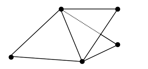

Why do we dislike non-manifolds? Unfortunately, I am not quite sure currently and this requires my further exploration.

Solution again: restricting each edge connecting maximum 2 faces.

Problem again again:
We can still get disconnected surface around vertex: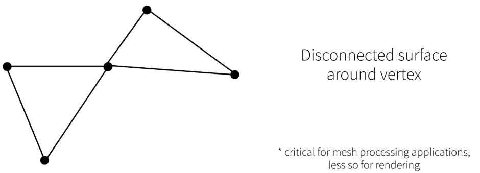

Maybe no solution
😭😭😭

Benefits of Triangular Meshes:

• Efficient to compute ray-triangle intersections
• Easy to texture and render(common representation across graphics)

  detailed principle may be covered in the future

Limitations:

• Simply editting shape by modifying vertex positions is trivial, while other changes are non-trivial. It's even more challenging when topology changes.

So if there an alternate representation that make topology-consistent changes easier?

Parametric Surfaces

Expression:

$$f(\textbf{u})=\textbf{p}\in \mathbb{R}^3;\textbf{u}\in \mathcal{M}$$

where $f$ is a continuous funtion over a 2D manifold $\mathcal{M}$ and it parametrizes a surface. The connectivity/topology is constrained to be same as $\mathcal{M}$.

Benefit： It disentangles discretization(vertices/faces) from shape representation. In triangular meshes, if we want to change shapes, we must change the connectivity of the vertices and faces. The resolution of meshes is tied with the shape. This method allows to change resolution without change shapes depending on how many $\textbf{u}$ you sample to feed into $f$. Since we just changes the samples in $\mathcal{M}$ instead of $f$, the shape keeps.

Idea: We can use neural network with parameters $\theta$ to get:

$$f_{\theta}(\textbf{u})=\textbf{p}\in \mathbb{R}^3;\textbf{u}\in \mathbb{S}^2$$

Limitations: Although it's easy to sample points on surface, it's hard to determine whether a query point $\textbf{q}$ is outside the shape (i.e. outside or inside the surface). It's also difficult to analytically render, since the computation of the ray-surface intersection is rather hard for arbitary $\textbf{f}$.

From surface representations to Volume representations

Since we have talked about point cloud,meshes and parametric surfaces. They all belong to surface representations. They have fundamental constraint: It's hard for them to know whether a point inside the object or not, how to fuse to objects and carve a section out of a solid object since they just model the surface of the object. In next sections, we will talk about volume representations which easily solve above problems. A fig briefly illustrates the differences: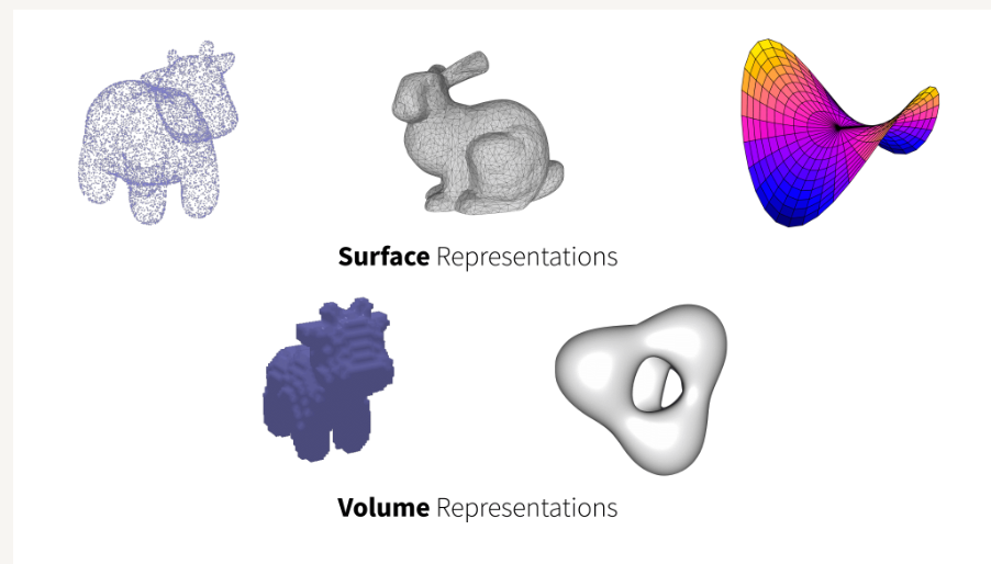

Voxelized 3D

We use a $(W\times H\times D)$ cuboid grid $V$ to contain the object. Each cell of grid object representing occupancy (or probability) at the cell:

$$V[x,y,z]\in [0,1]$$

Coding tips: you can use cuboid endpoints (i.e. $(x_{\min},y_{\min},z_{\min},x_{\max},y_{\max},z_{\max})$ to represent a cell's coordinate); you can also disentangle grid coordinates with real position by implementing a transformation function.

Limitation: It's computationally challenging to scale resolution (grows cubically).

Implicit Surfaces

Main idea: Use the zero crossing of a continuous function $\textbf{f}$ to parametrize a surface:

$$\{\textbf{p}\mid f(\textbf{p})=0\}$$

$\textbf{f}$ can be anything--- a simple function, or a NN.

Some properties:

• Easy boolean operations: $$\begin{aligned} & \cup_if_i(\textbf{p})=\min_{i}f_i(\textbf{p}) \quad (\text{Union of objects})\\ & \cap_if_i(\textbf{p})=\max_{i}f_i(\textbf{p}) \\ &(f-g)(\textbf{p})=\max (f(\textbf{p},-g(\textbf{p}))) \end{aligned}$$ where $f_i(\textbf{p})>0$ if $\textbf{p}$ is outside the object.
  We can also use NN with parameter $\theta$: $\{\textbf{p}\mid f_{\theta}(\textbf{p})=0\}$
• Signed Distance Function:Additional condition can be applied to $f$: let$f(\textbf{p})$ represent (signed) distance to surface from point $\textbf{p}$. SDF satisfy: $||\nabla f||=1$ which will be covered in future sections.
• Harmonic Functions: Addtional condition as SDF can be applied to $f$: $\nabla. \nabla f=0$ which will also be covered in future sections.

Limitations: Although it's easy to answer questions about occupancy, it's difficult to reason about the surface (may not even exist given an arbitraty $f$).

Density field

In density field, there is no notion of a surface(e.g. $f(\textbf{p})=0.1$ everywhere can represent a semi-transparent fluid)

We will revisit it in more details.

Conversions across different representations

Let's first formally define this problem: we have two representations each with parameters $\theta_1$ and $\theta_2$. We want to find a differentiable transformation $\mathcal{T}$ from representation1 to representation2:

$$\begin{aligned} \theta_2=\mathcal{T}(\theta_1) \end{aligned}$$

We can use the idea from back-propagation:

$$\begin{aligned} \text{input(e.g. image)} \xrightarrow{f_{\theta_1}} \text{representation1} &\xrightarrow{f_{\theta_2}}\text{representation2} &\rightarrow \mathcal{L}(\text{loss, a scaler})\\ & \color{red}{\leftarrow \frac{\partial \mathcal{L}}{\partial \theta_2}\cdot\frac{\partial \theta_2}{\partial \theta_1} }& \color{red}{\leftarrow} \frac{\partial \mathcal{L}}{\partial \theta_2} \end{aligned}$$

So if we can compute $\frac{\partial \theta_2}{\partial \theta_1}$， then we can get $\mathcal{T}$ by back-propagation.

Conversions within volume representation

Let's begin by Conversions within volume representation. There are discrete representaion, e.g. voxelized 3D and continuous representation, e.g. implicit surfaces.

From discrete to continuous

The method is quite simple: interpolation. If $V$ (the grid of voxels) $\in \mathbb{R}$,then use Linear Interopolatoin to estimate continuous function $f$. If $V \in \mathbb{R}^2$, then Bilinear Interpolation. If $V \in \mathbb{R}^3$, then Trilinear Interpolation

From continuous to discrete

Suppose we have continuous representation:

$$\begin{aligned} \{ \textbf{p}\mid f(\textbf{p})=0\} \end{aligned}$$

We want to transform it to discrete representation:

$$\begin{aligned} V[\textbf{p}] \in [0,1]\\ \textbf{p}\in \text{grid } \mathcal{G} \end{aligned}$$

We evaluate $f$ for all points in the grid. We set $V[\textbf{p}]=sgn(f(\textbf{p}))$ or $V[\textbf{p}]=sigmoid(f(\textbf{p}))$. Since by the difinition of implicit surfaces: $f(p)>0$ if p is inside the surface, so we can set $V[\textbf{p}]=1$ or high probability.

However, to easily compute $\frac{\partial V[\textbf{p}]}{\partial f(p)}$, we often set $V[\textbf{p}]=sigmoid(f(p))$

Conversions within surface representation

From continuous to discrete

Suppose we have parametric surfaces:

$$\begin{aligned} f(\textbf{u})&=\textbf{p}\in \mathbb{R}^3\\ \textbf{u}&\in \mathcal{M} \end{aligned}$$

We want to discretize it to meshes. The discretization of this process is to sample some vertices and faces that construct the meshes. The derivatives of vertex positions w.r.t can be computed, but face not. Solution is we predefine the connectivity in $\mathcal{M}$. We firstly discretize $\mathcal{M}$, get verties and face connectivity information. Then feed these sampled points to $f$ while reserving the connectivity. Thus we obtain the meshes representations.

Sample points on a triangle mesh

Three ways:

• uniformly sample triangle and uniformly sample a point in the triangle
• with area-proportional probability and uniformly sample a point on the triangle
• Select a point furthest from the current set

Volumes to Surface

We are given an input: continuous values at each cell in a discrete grid. We want the output: surface meshes.
We assume that each cell in the grid stores a value with surface being zero-crossing. How do we get the surface meshes?

Solution: use Marching Squares (2D case)link or Marching Cubes (3D case) link

Points to Meshes

It's non-trivial to define connectivity rules since the point clouds are not robust to noise. Thus directly adding edges in point clouds may not work.

Key idea: from above section, we see it's feasible to transform volumes to surface. So if we can first transform the point clouds to volume representation, then we can indirectly get meshes.

Key idea again: Points represent (noisy) samples from zero-level set of an implicit function since each point in point clouds can be noisly regard as the surface of the object. So instead of directly trying to add triangles, we can optimize an implicit function instead.

Problem: In ml, predicting a constantly-zero implicit function may result in a constantly-zero function.

Solution: We can use oriented point clouds. That is, we append each point's normal vector to the point clouds' representaion. This method is also called Possion Reconstruction

Poisson Reconstruction

Key idea: Find a (smoothed) indicator function whose gradient corresponds to the surface normals.

A smoothed indicator function is not a strict binary function: inside the object, its value is 1 or near 1; outside the object, its value is 0 or near 0. From outside to inside, its values smoothly and continuously range from 0 to 1.

Thus we can use the iso-surface (i.e. indicator function at the points in this surface has value 0.5) of the indicator function to estimate the actual surface.

I won't cover the calculation details since this blog is just an overview. If interested, see here.