The goal of fitting is to find a parametric model (e.g. line, curve) that best describes the observed data. We can obtain the optimal paramters of the model by minimizing a fitting error r betwee the data and a particular estimate of the model parameters.
I will introduce three techniques:
- Least-squares
- RANSAC (random sample consensus)
- Hough transform
Least-squares
Naive way
Maybe you have been quite familiar with the problem: Given a series of $N$ 2D points $\{(x_i,y_i)\}_{i=1}^N$, you need to find a line $y=mx+b$ such that the squared error in the $y$ dimension is minimized.
Specifically, we want to find model parameters $w=[m\quad b]^T$ to minimize error function $E$:
We then set the gradient of the error function $E$ w.r.t $w$ equal to 0:
Thid leads to the normal equations:
We assume that $X$ is full-rank, so $X^TX$ is invertible. Thus we get a closed-form solutoin for $w$:
Improvement
However, this method fails completely for fitting points that describe a vertical line ($m$ undefined). In this case, $m$ would be set to extremely large, leading to numerically unstable solutions. So we can use an alternate line formulation of the form:
Note that our new line parameterization accounts for error in both the $x-$ and $y-$axes, our new error is the sum of squared orthogonal distances.
Given a 2D data point $P=(x_i,y_i)$, its distance from the line is:
To simplify, we constrain the normal vector $||\vec{\textbf{n}}||=\sqrt{a^2+b^2}=1$
Thus, the new erro function $E$ is:
where $a^2+b^2=1$.
Since we notice that $E(a,b,c)$ is convex w.r.t parameter $c$. We can first fix $(a,b)$ and compute the optimal $c$ by setting the gridiant of $E$ w,r,t $c$ equal 0:
We get $c=-a\overline{x}-b\overline{y}$
As we get $c$, we can rewrite $E$:
We can easily get the optimal $w$ by using $\textbf{SVD}$ on $X$:
$\hat{w}$ is the lost column of $V$
If you are not familiar with $\textbf{SVD}$, I strongly recommend reading this to have a thorough understanding since $\textbf{SVD}$ is a common techniques in computer vision.
Further improvement:
In practice, least-squares fits noisy data well but is susceptible to outliers. If we write the residual for $i$-th data point as $r_i=ax_i+by_i+c$ and the cost as $C(r_i)=r_i^2$. The quadratic growth of the squared error $C(r_i)$ means that outliers with large residuals $r_i$ exert an outsized influence on cost minimum.
We can penalize large residuals less by a robust cost function:
A larger $\sigma$ widens the quadratic curve in the center, penalizing outliers more relative to other points (similar to the original squared error function). A small $\sigma$ narrows the quadratic curve, penalizing outliers less.If $\sigma$ is too small, then most of the residuals will be treated as outliers even when they are not, leading to a poor fit. If $\sigma$ is too large, then we do not benefit from the robust cost function and end up with the least-squares fit.
Since the robust cost functions are non-linear, they are optimized with iterative methods. In practice, the closed-form least-squares solution is often used as a starting point, followed by iteratively fitting the parameters with
a robust non-linear cost function.
RANSAC
This method, which stands for random sample consensus, is designed to be robust to outliers and missing data. I will show how to use this to perform line fitting, but it generalizeds to many different fitting contexts.
Alogorithm process
Given a series of $N$ 2D points $X=\{(x_i,y_i)\}_{i=1}^N$ that we want to fit a line to, the process is:
- First, randomly select the minimum number of points needed to fit a model. A line requires at least two points, so we randomly chooes two.
- Fit the model to the randomly selected sample set.
- Use the fitted model to compute the inlier set from the entire dataset. Given the model parameters $w$, it's defined by:where $r$ is the residual between a data point and the model and $\delta$ is some arbitrary threshold. So the outlier set is defined by $O=X \backslash P$.
- We repeat these steps for a finite number of iterations $M$ with a new random sample each time until the size of the inlier set is maximized.
Tune parameters
The number of times to sample $n$ and the tolerance threshold $\delta$ need to predifine before the algorithm. It's unnecessary to try every possible sample.We can estimate the number of iterations $n$ to guarantee with probability $p$ at least one random sample with an inlier set free of “real” outliers for a given $s$ (minimum number
of points required to fit a model) and $\epsilon $ ∈ [0, 1] (proportion of outliers):
- The chance that a single random sample of $s$ points contain all inliers is $(1-\epsilon)^s$
- The chance that a single random sample contains at least one outlier is $1-(1-\epsilon)^s$
- The chance that all $n$ samples contain at least one outlier is $(1-(1-\epsilon)^s)^n$
- the chance that at least one of the $n$ samples doesn't contain ant ouliers is $p=1-(1-(1-\epsilon)^s)^n$
Thus we can derive $n$:
Hough Transform
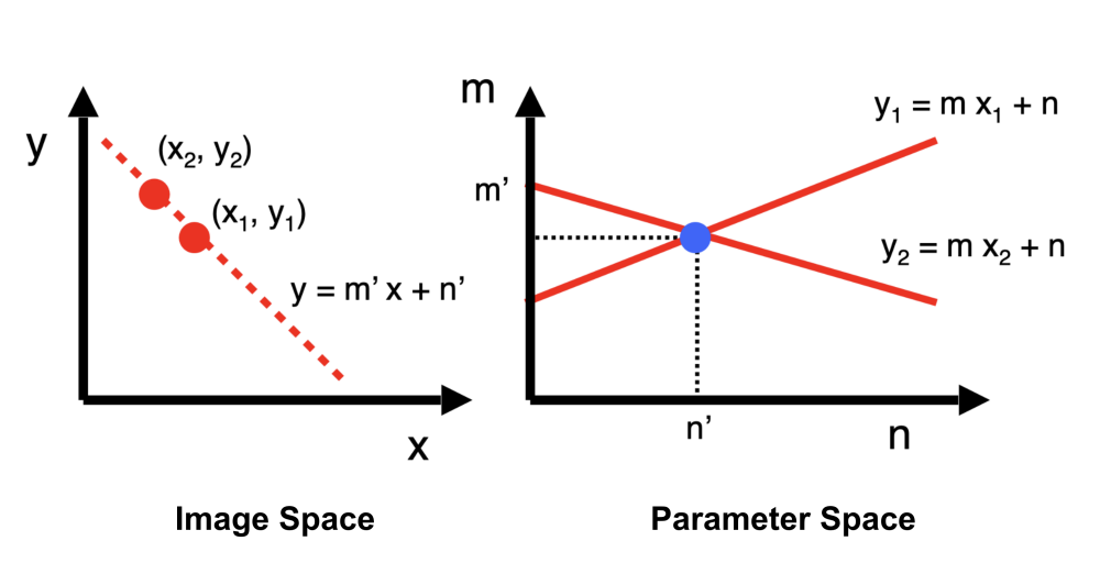
The problem is the same as before. This method considers dull parameter, or $\textbf{Hough space}$. A point in the image space (on the line $y_i=mx_i+n$) becomes a line in the parameter space defined by $n=-x_im+y_i$. Similarly, a point in the parameter space ($m,n$) is a line in the image space given by $y=mx+n$. As illustrated:
We see that a line in the parameter space $n=-x_im+y_i$ represents all of the different possible lines in the image space that pass through the point $(x_i,y_i)$ in the image space. Thus, to find the line in the image space that fits both image points $(x_1,y_1)$ and $(x_2,y_2)$, we associate both points with lines in the Hough space and find the point of intersection $(m',n')$.
In practice, we divide the Hough space into a discrete grid of squared cells with width $w$ for the parameter space. We maintain a grid of counts for every $w\times w$ cell centered at $(m,n)$ denoted as $A(m,n)=0$ for all $(m,n)$ initially. For every point ($x_i,y_i$) in the image plane, we find all $(m,n)$ satisfying $n=-x_im+y_i$ and increment the count by 1. After we do for all data points, the point $(m,n)$ in Hough space with highest count represent the fitted line in the image plane.
However, as Least-squares case, $m$ is unbounded which make this method computational and memory intensive.
Polar Parameterization Improvement
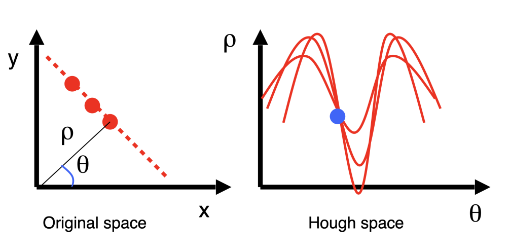
To solve this, we can consider a solar parameterization of a line:
$$
x\cos (\theta) + y \sin (\theta)=\rho
$$, as illustrated:
From the fig, we see that $\rho$ is the distance from the origin to the line (bounded by the image size) and that $\theta$ is the angle between the x-axis and and normal vector of the line (bounded between 0 and $\pi$). So we can use the same voting strategy to get the best $\theta$ and $\rho$.
In practice, noisy data points means that sinusoidal profiles in the Hough space that correspond to points on the same line in the image space, may not necessarily intersect at the same point in the Hough space. To slove this we can increase the width $w$ of the grid cells, which increases the tolerance to imperfect intersections. So small grid sizes may result in missed image space lines due to noise, while large grid sizes may merge different lines and reduce estimation accuracy since all $\rho,\theta$ within a cell are possible lines.